Simulating Lasers

Spent a Friday evening getting my head stuck down this rabbit hole...

Motivation

I used to do a fair amount of computational physics back when I was a first or second-year physics student (at the University of Manchester) many years back, and I have some fond (and slightly painful) memories of trying to simulate the behaviour of a laser in a computer lab, wrestling with structs and pointers (in plain-old C) alongside Greg, my trusty lab partner. I fear most of that work is now lost or buried in a dusty loft somewhere, and for some reason it crept back into my mind while I was ideating on this site. So I decided to arm myself with some AI-assisted learning and try to recreate the project; vague flashbacks have since sharpened into much clearer memories.

Physical picture

This walkthrough assumes some basic starting knowledge and concepts:

Energy levels and populations

• Atoms/ions in the gain medium have discrete energy levels: $E_0$, $E_1$, $E_2$, ...
• A population $N_i​(t)$ is the number (or density) of atoms in level $i$ at time $t$.
• In thermal equilibrium, most atoms sit in the lowest level (ground state).

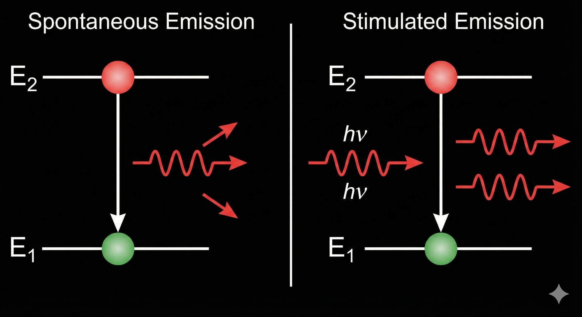
Stimulated vs spontaneous emission

• An excited atom is basically where one of it's electrons is temporarily in an excited and elevated state. It can be kicked there by absorbing a photon, and can relax by emitting another photon.
• Spontaneous emission: an excited atom randomly emits a photon and drops down (no external light needed).
• Stimulated emission: an incoming photon of the right frequency triggers an excited atom to drop down and emit a second photon in phase and same direction → this is the laser process.
• To get net gain, you need a population inversion: more atoms in the upper laser level than in the lower one.

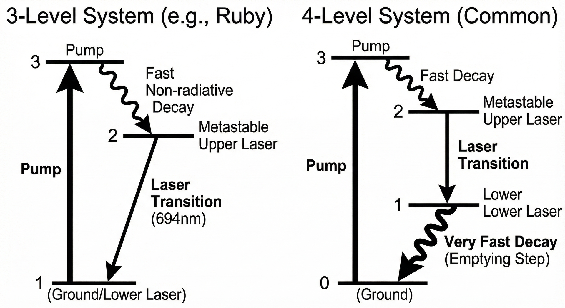
In a simple 3-level laser (e.g. a solid-state ruby crystal), there's:

• a ground-state, $E_0$ with the lowest energy
• a "metastable" state $E_1$, which basically means atoms can sit around in for a reasonable amount if time and either decaying sponaneiously or stimulated by a passing photon
• an upper high-energy state $E_2$, which wants to decay rapidly and spontaneously to $E_1$

Kick a bunch of atoms from $E_0$ to $E_2$ and they'd rapidly decay to $E_1$, and hang around for a bit; and when there's more in $E_1$ than $E_0$, we call this a population inversion.

Here’s a more detailed diagram showing the same thing, and what a 4-level laser system might look like (thanks Gemini for these!):

A simple schematic of a laser is shown here; the lasing medium (e.g. a ruby crystal) is capped between two mirrors, one ever so slightly transparent and letting through ~1% of the light (the laser beam):

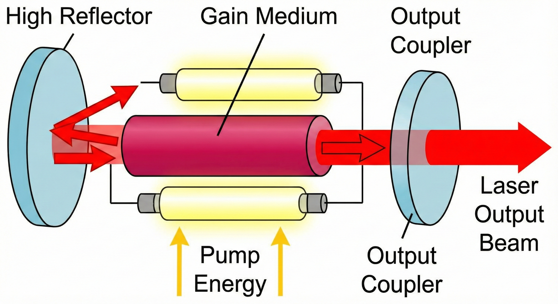
You put the energy in by “pumping”, typically one of the following ways:

• optical
• electrical
• chemical
• nuclear
• ...

We’ll keep things simple here and consider optical pumping: using light. You shine strong light (from a flashlamp or laser diode) into the crystal. That light has the right wavelengths to excite electrons from the ground state to a higher level.

From basic physics to equations

Now for the maths. Here’s a standard, reasonably simple 3-equation model we used.

Variables

• $N_2(t)$: population in the upper laser level
• $N_1(t)$: population in the lower laser level
• $S(t)$: photon number in the cavity mode (or proportional to intensity)

Parameters

• $R$: pump rate into the upper laser level (atoms per second). This is what we will sweep to represent “pump power”.
• $\tau_{21}$: lifetime of level 2 (2 → 1, spontaneous/non-radiative)
• $\tau_{10}$: lifetime of level 1 (1 → ground), often fast in a 4-level system
• $G$: stimulated emission coefficient, coupling between inversion and photon number
• $\Gamma$: confinement/overlap factor (how well the light overlaps the gain medium)
• $\beta$: spontaneous emission factor into the laseing mode (0–1)
• $\tau_p$: photon lifetime in the cavity (mirror losses, scattering, output coupling)

Model equations

$\boxed{ \begin{aligned} \frac{dN_2}{dt} &= R - \frac{N_2}{\tau_{21}} - G \bigl(N_2 - N_1\bigr)S \\ \frac{dN_1}{dt} &= \frac{N_2}{\tau_{21}} + G \bigl(N_2 - N_1\bigr)S - \frac{N_1}{\tau_{10}} \\ \frac{dS}{dt} &= \Gamma G \bigl(N_2 - N_1\bigr)S + \beta \frac{N_2}{\tau_{21}} - \frac{S}{\tau_p} \end{aligned} }$

Now term-by-term:

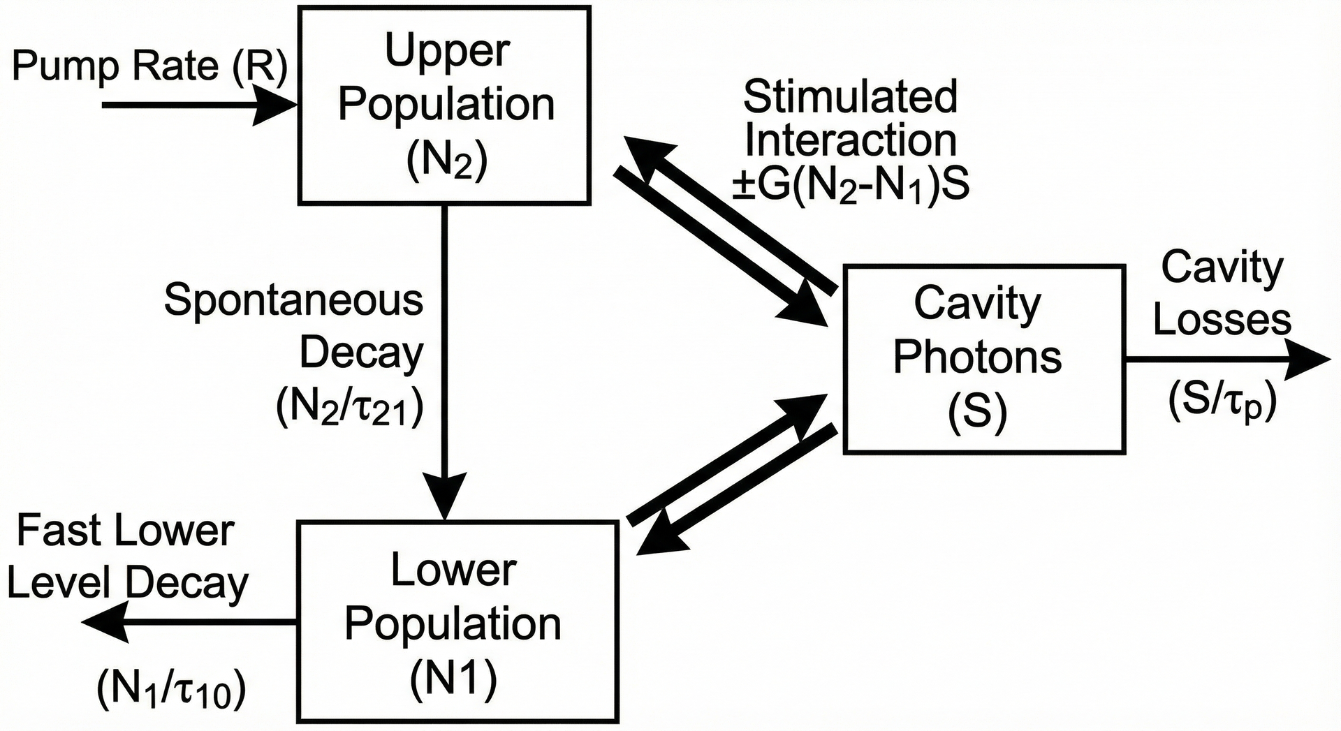
Upper level $N_2$

$\boxed{ \begin{aligned} \frac{dN_2}{dt} = R - \frac{N_2}{\tau_{21}} - G (N_2 - N_1) S \end{aligned} }$

• $+R$: external pump populates level 2. − $N_2\tau_{21}$: level 2 decays spontaneously to level 1.
• $−G(N_2−N_1)S$: stimulated transitions driven by photons in the cavity.
  • If $N_2$ > $N_1$, this is mostly stimulated emission 2→1 (depletes $N_2$).
  • The factor $N_2 - N_1$ is essentially inversion.

Lower level $N_1$

$\boxed{ \begin{aligned} \frac{dN_1}{dt} = \frac{N_2}{\tau_{21}} + G (N_2 - N_1) S - \frac{N_1}{\tau_{10}} \end{aligned} }$

• Gains population from upper level via spontaneous and stimulated emission.
• Loses population to the ground (for a 4-level laser this is a fast “dumping” process).

Photon number $S$

$\boxed{ \begin{aligned} \frac{dS}{dt} = \Gamma G (N_2 - N_1) S + \beta \frac{N_2}{\tau_{21}} - \frac{S}{\tau_p} \end{aligned} }$

• Stimulated term: the inverted medium acts as an amplifier.
• Spontaneous term: “seed” photons injected into the mode.
• Loss term: photons leak out or are absorbed.

This is nonlinear (because of the $(N_2 - N_1)S$ terms) and fully coupled. It’s rich enough for nice physics: threshold, relaxation oscillations, transient behaviour, the effect of slow or fast depopulation of the lower level, etc.

Don’t worry too much about where these equations come from, but know that they make intuitive sense. For example: the rate of change of atoms in level $E_2$ ($\frac{dN_2}{dt}$) is related to the energy you’re pumping in ($+R$), minus those leaving to the lower level by either spontaneous decay to level 1 ($-,N_2/\tau_{21}$) or stimulated emission ($-,G(N_2 - N_1)S$).

Here’s a schematic illustration of the equations and their main terms, showing the flows of atoms to and from each state.

Numerical method

Now we have the setup, it’s on to the fun part where we attempt to solve the equations and then interpret the results!

But first, why do we actually need to solve the equations, and what does that actually mean. In many cases in physics, it is relatively easy to describe a system in differential form; e.g. understanding the processes in terms of rate of change of something, rather than the something itself. (Some situations it's easier to do things in terms of its integral form, but that's for another day). Many differential equations have closed-form "analytical" solutions where you can solve them exactly, and the above equations do have some simple cases which can be solved analytically, namely:

• the trivial case where everything is zero, and
• the steady-state case, where the rates-of-changes are all zero.

But if we want to know the more interesting cases, and we wish to be able to describe e.g. the photon density at any point in time, we need to solve the equations. Non-linear equations famously don't have easy analytical solutions, so we must resort to more brute-force numerical approximations.

There are many numerical methods to pick from for integrals and differential equations. Integration is conceptually a little easier to visualize, as it’s just like finding the area under a curve, often by approximating the curve with straight lines (so computing the area is trivial). For differential equations, we’re going to use a method called the Runge–Kutta method (RK4).

Think of it like this: there is a function whose differential form we know. A differential is like the slope of a curve, so if we know the local slope of the curve and we know where we are, we work out the current value and can then inch along to map out what the function looks like. A differential equation tells you how fast something is changing right now. A numerical method like RK4 uses that local “how fast” information to step forward in time, over and over, to trace out what happens. If the slope is steep, we take smaller steps to stay on track.

Wikipedia has a good overview of the RK4 algorithm: we compute the slopes at four points around a specific point, then compute a weighted average to get a better estimate of the function before incrementing.

Here's a simple implementation...

We can define a state vector we wish to know,

So $y(t)$ has the detail about the 3 populations. We define a function $f(t,y)$ that returns $\frac{dy}{dt}$ like this:

def f(t, y, params):
    N2, N1, S = y
    R, tau21, tau10, G, Gamma, beta, tau_p = params

    dN2 = R - N2/tau21 - G*(N2 - N1)*S
    dN1 = N2/tau21 + G*(N2 - N1)*S - N1/tau10
    dS  = Gamma*G*(N2 - N1)*S + beta*(N2/tau21) - S/tau_p

    return np.array([dN2, dN1, dS])

We can then define an RK4 step as:

def rk4_step(t, y, dt, f, params):
    k1 = f(t,          y,               params)
    k2 = f(t + dt/2.,  y + dt*k1/2.,    params)
    k3 = f(t + dt/2.,  y + dt*k2/2.,    params)
    k4 = f(t + dt,     y + dt*k3,       params)
    return y + dt*(k1 + 2*k2 + 2*k3 + k4)/6.

We can then loop over time; at each step store $t$, $N_1$, $N_2$, $S$ (e.g. in arrays or a pandas DataFrame). Here's a simple loop to solve the equations iteratively:

t0, t_end, dt = 0.0, 10.0, 0.001
times = []
states = []
t = t0
y = np.array([N2_0, N1_0, S_0])
while t <= t_end:
    times.append(t)
    states.append(y.copy())
    y = rk4_step(t, y, dt, f, params)
    t += dt

Expectations

Based on some hazy memories, there’s a critical threshold of energy needed to start lasing. Below this, the energy just dissipates and you mostly end up warming the thing up. But at a specific input energy level, the system starts to lase and throw out a beam. From then on, the more energy you pump in, the stronger the laser becomes. So we’re expecting a hockey-stick type curve: initially flat, then roughly linear after a certain point.

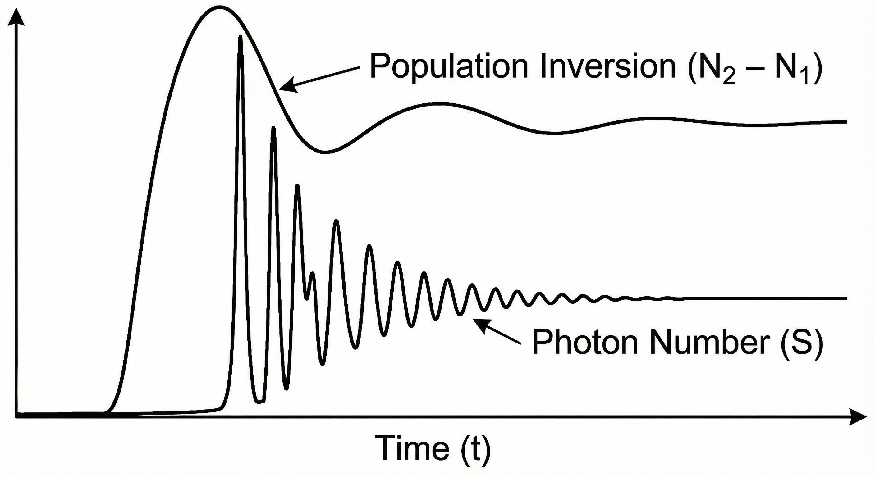
Because it’s a non-linear system, there should also be some nice dynamic oscillations, instabilities, resonances, etc. as the pump is suddenly switched on above threshold and everything starts to stabilise. Seeing something like this in the simulation would be a nice outcome.

Results

I used the GPT-suggested unitless parameters as follows:

{
    "tau21": 1.0,   # upper level lifetime
    "tau10": 0.1,   # lower level lifetime (fast dump to ground)
    "tau_p": 0.1,   # photon lifetime in the cavity
    "G": 1.0,       # stimulated emission coefficient
    "Gamma": 1.0,   # overlap / confinement factor
    "beta": 0.01,   # spontaneous emission into the lasing mode
}

Threshold curve

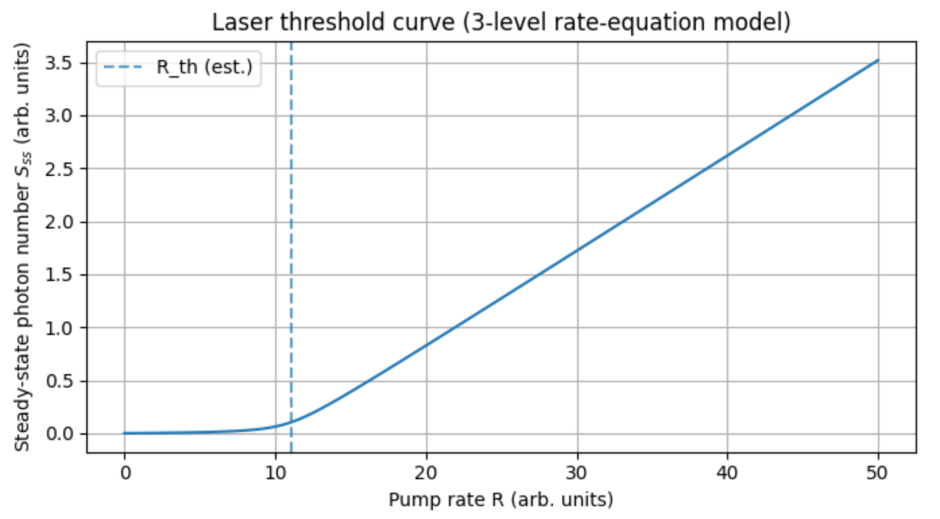
Here we clearly see the threshold pumping power ~ 11, with approx linear relationship after, closely matching predictions

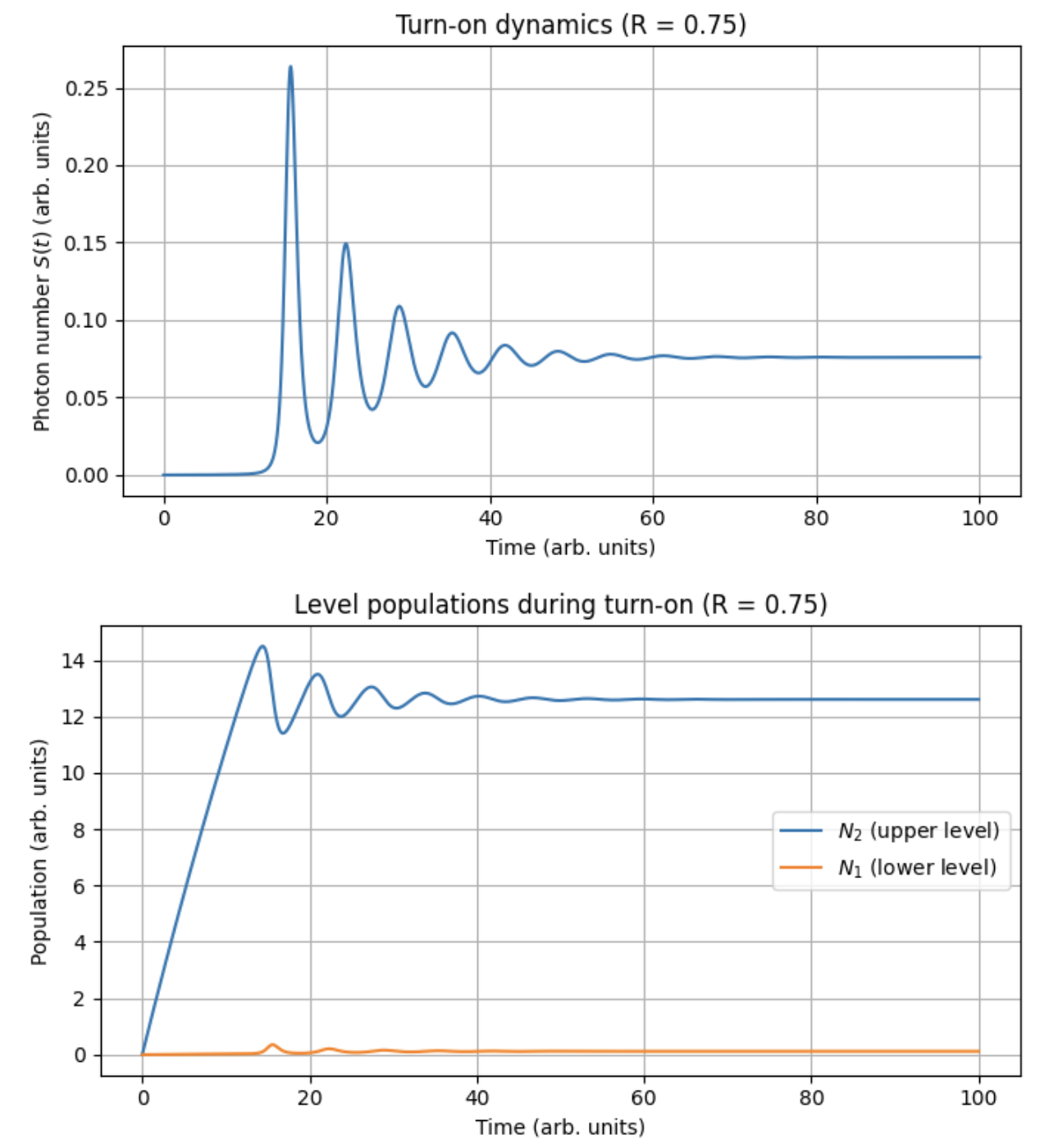
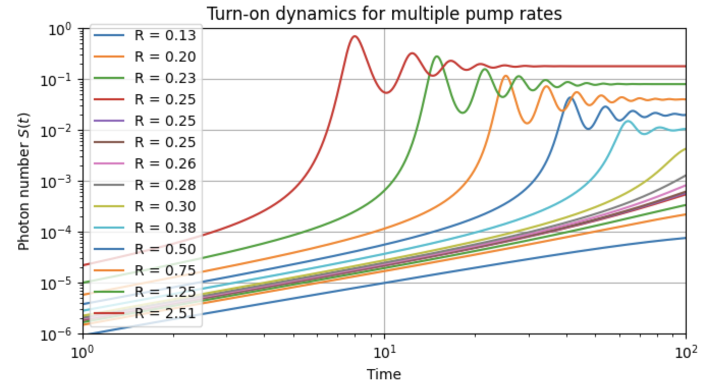
Turn-on dynamics

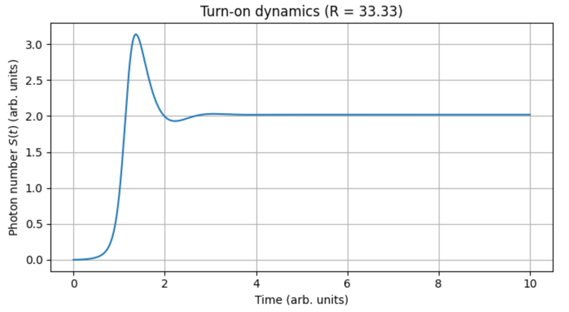
Randomly picking a pumping power well above the threshold (30), we can clearly see the power of the laser oscillate and stablise. Looks like a nearly-critically-damped oscillation; I wonder if selecting a value nearer or well above the threshold would show a more dynamic over/undershooting?

Level populations

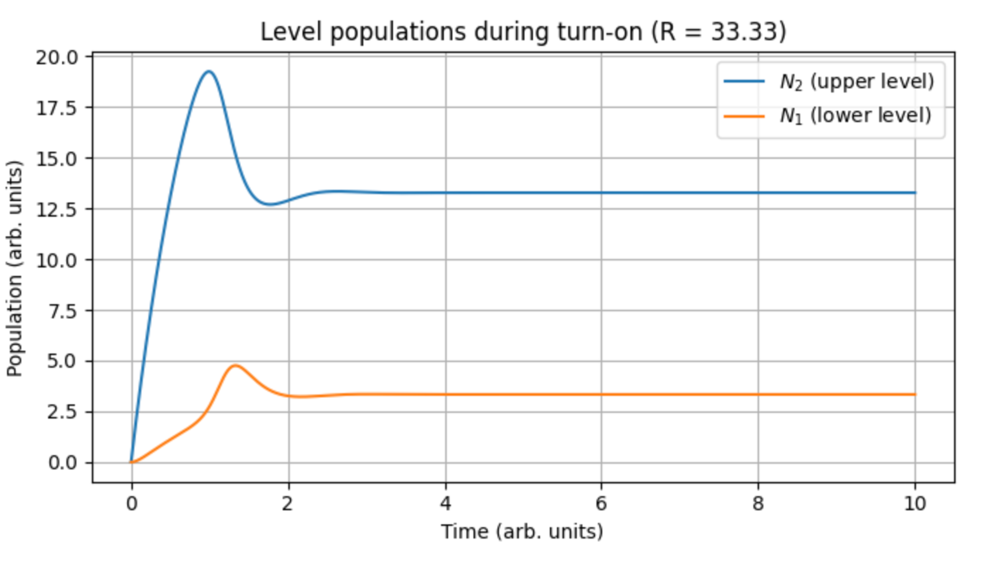
Here we can visualise the number of atoms in each level/population over time

What I learned

• I actually remember far more that I thought I did. Just a few little nudges needed but still there. I've not even thought of the Runge-Kutta algorithm in the last 20 years!
• ChatGPT did great at synthesising a learning plan, and Gemini did great at the images.
• AI aside, computational physics is soooo much easier these days, even without specialised libraries. I don't miss C and Matlab, to be honest.
• Dimensional analysis makes things a lot cleaner and simpler using unitless parameters

Further work

• Research chemical lasers, and microwave lasers (MASERS) for any other interesting physics
• Modulate the pump as $R(t) = R_0 ​+ \Delta R cos(\omega t)$
• Two-mode competition: Extend from one $S(t)$ to $S_1(t), S_2(t)$ to show how two cavity modes can compete for the same inversion.
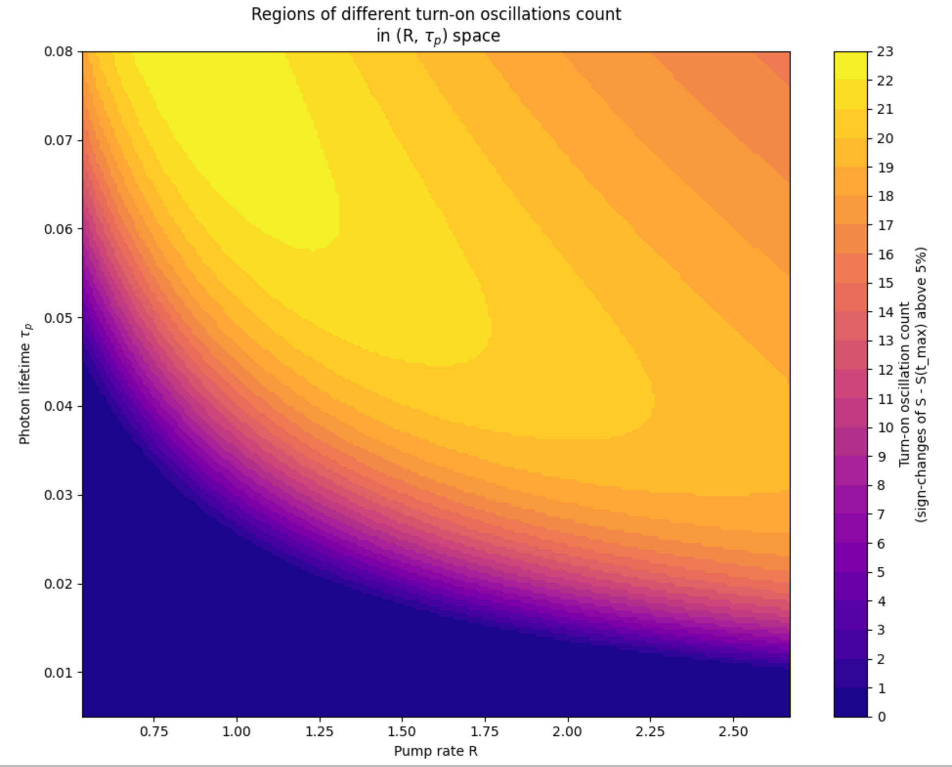
• Plot phase diagrams showing areas of no lasing, steady lasing and strong oscillations, by plotting $R$ against $\tau_p$

Addendum

Final script

import numpy as np
import pandas as pd
import matplotlib.pyplot as plt

# -----------------------------
# Laser rate-equation parameters
# -----------------------------
# Time units are arbitrary (you can think of them as microseconds if you like).
# Values are chosen to give a visible threshold and nice turn-on dynamics.
params = {
    "tau21": 1.0,   # upper level lifetime
    "tau10": 0.1,   # lower level lifetime (fast dump to ground)
    "tau_p": 0.1,   # photon lifetime in the cavity
    "G": 1.0,       # stimulated emission coefficient
    "Gamma": 1.0,   # overlap / confinement factor
    "beta": 0.01,   # spontaneous emission into the lasing mode
}

# Approximate threshold pump rate (from linear analysis around S ~ 0)
tau21 = params["tau21"]
tau10 = params["tau10"]
tau_p = params["tau_p"]
G = params["G"]
Gamma = params["Gamma"]
R_threshold_est = 1.0 / ((tau21 - tau10) * Gamma * G * tau_p)

R_turn_on = 1.5 * R_threshold_est  # try 1.5–2.0×, not 3×


print(f"Approximate threshold pump rate R_th ≈ {R_threshold_est:.2f}")


# -----------------------------
# Right-hand side of ODE system
# -----------------------------
def laser_rhs(t, y, R, p):
    """
    Right-hand side of the 3-level laser rate equations.

    y = [N2, N1, S]
      N2 : upper level population
      N1 : lower level population
      S  : photon number in the lasing mode
    R = pump rate
    p = parameter dict
    """
    N2, N1, S = y
    tau21 = p["tau21"]
    tau10 = p["tau10"]
    tau_p = p["tau_p"]
    G = p["G"]
    Gamma = p["Gamma"]
    beta = p["beta"]

    # Rate equations
    dN2 = R - N2 / tau21 - G * (N2 - N1) * S
    dN1 = N2 / tau21 + G * (N2 - N1) * S - N1 / tau10
    dS = Gamma * G * (N2 - N1) * S + beta * N2 / tau21 - S / tau_p

    return np.array([dN2, dN1, dS], dtype=float)


# -----------------------------
# RK4 integrator
# -----------------------------
def rk4_step(fun, t, y, dt, *args, **kwargs):
    """Single Runge–Kutta 4 step."""
    k1 = fun(t, y, *args, **kwargs)
    k2 = fun(t + dt / 2.0, y + dt * k1 / 2.0, *args, **kwargs)
    k3 = fun(t + dt / 2.0, y + dt * k2 / 2.0, *args, **kwargs)
    k4 = fun(t + dt, y + dt * k3, *args, **kwargs)
    return y + dt * (k1 + 2 * k2 + 2 * k3 + k4) / 6.0


def simulate_time_series(R, t_max, dt, p, y0=None):
    """
    Integrate the laser system for a given pump rate R.

    Returns:
        t : array of times, shape (n_steps+1,)
        y : array of states [N2, N1, S], shape (n_steps+1, 3)
    """
    n_steps = int(np.ceil(t_max / dt))
    t = np.linspace(0.0, n_steps * dt, n_steps + 1)

    y = np.zeros((n_steps + 1, 3), dtype=float)
    if y0 is None:
        y[0] = np.array([0.0, 0.0, 0.0], dtype=float)
    else:
        y[0] = np.array(y0, dtype=float)

    for i in range(n_steps):
        y[i + 1] = rk4_step(laser_rhs, t[i], y[i], dt, R, p)

    return t, y


def steady_state_S(R, p, t_max=15.0, dt=0.003, tail_fraction=0.3):
    """
    Run the system and estimate steady-state photon number S.

    We average S over the last `tail_fraction` of the time series to
    smooth out any small residual oscillations.
    """
    t, y = simulate_time_series(R, t_max=t_max, dt=dt, p=p)
    S = y[:, 2]
    n = len(S)
    tail_start = int((1.0 - tail_fraction) * n)
    return S[tail_start:].mean()


# -----------------------------
# 1. Threshold curve
# -----------------------------
R_values = np.linspace(0.0, 50.0, 100)  # pump range to explore
S_ss_values = [steady_state_S(R, params) for R in R_values]

threshold_df = pd.DataFrame({
    "R": R_values,
    "S_ss": S_ss_values,
})

fig, ax = plt.subplots(figsize=(7, 4))
ax.plot(threshold_df["R"], threshold_df["S_ss"])
ax.axvline(R_threshold_est, linestyle="--", alpha=0.7, label="R_th (est.)")
ax.set_xlabel("Pump rate R (arb. units)")
ax.set_ylabel("Steady-state photon number $S_{ss}$ (arb. units)")
ax.set_title("Laser threshold curve (3-level rate-equation model)")
ax.grid(True)
ax.legend()
plt.tight_layout()
plt.show()


# -----------------------------
# 2. Turn-on dynamics
# -----------------------------
# Choose a pump rate above threshold (roughly ~2–3× threshold)
R_turn_on = 3.0 * R_threshold_est
print(f"Simulating turn-on dynamics for R = {R_turn_on:.2f}")

t_dyn, y_dyn = simulate_time_series(R_turn_on, t_max=10.0, dt=0.001, p=params)

dyn_df = pd.DataFrame({
    "t": t_dyn,
    "N2": y_dyn[:, 0],
    "N1": y_dyn[:, 1],
    "S":  y_dyn[:, 2],
})

# Photon number vs time (shows turn-on and relaxation oscillations)
fig, ax = plt.subplots(figsize=(7, 4))
ax.plot(dyn_df["t"], dyn_df["S"])
ax.set_xlabel("Time (arb. units)")
ax.set_ylabel("Photon number $S(t)$ (arb. units)")
ax.set_title(f"Turn-on dynamics (R = {R_turn_on:.2f})")
ax.grid(True)
plt.tight_layout()
plt.show()

# Level populations vs time
fig, ax = plt.subplots(figsize=(7, 4))
ax.plot(dyn_df["t"], dyn_df["N2"], label=r"$N_2$ (upper level)")
ax.plot(dyn_df["t"], dyn_df["N1"], label=r"$N_1$ (lower level)")
ax.set_xlabel("Time (arb. units)")
ax.set_ylabel("Population (arb. units)")
ax.set_title(f"Level populations during turn-on (R = {R_turn_on:.2f})")
ax.grid(True)
ax.legend()
plt.tight_layout()
plt.show()

Oh - and if you got this far and if you didn't already know, laser is an acronym so should actually be written LASER: “Light Amplification by Stimulated Emission of Radiation”.